
Table of Contents >> Show >> Hide
- What “Transpose” Means in Excel (and When You Actually Need It)
- Method 1: Paste Special → Transpose (Fast One-Time Flip)
- Method 2: TRANSPOSE() Function (The “Live Link” Option)
- Method 3: Power Query Transpose (Repeatable, Great for Messy Imports)
- Troubleshooting: Why Your Horizontal-to-Vertical Transpose “Didn’t Work”
- Pro Tips for Cleaner Results (and Fewer Spreadsheet Regrets)
- Conclusion
- Real-World Transpose Stories (and What They Teach)
- SEO Tags
If your Excel data is laid out horizontally (across columns) but needs to be vertical (down rows), you don’t have to retype anything. You just need to transpose itaka rotate the range 90 degrees like your spreadsheet is doing a gentle yoga twist.
In this guide, you’ll learn the three most practical ways to transpose in Excel (including shortcuts), when to use each one, and how to avoid the classic “Why did Excel just eat my formatting?” moment.
What “Transpose” Means in Excel (and When You Actually Need It)
Transpose is Excel’s word for swapping rows and columns. A row of values becomes a column, and a column becomes a row. It’s perfect when:
- You copied data from a report laid out across the top (months, quarters, survey answers, etc.)
- You need a vertical list for a dropdown, chart, PivotTable, or import template
- You want to flip a small table so the labels run down the left side instead of across the top
Quick note: transposing is different from PivotTables or Power Query “Unpivot”. Pivoting/unpivoting reshapes data into a database-friendly format. Transpose is a literal row/column flip. Simple, direct, and occasionally dramatic.
Method 1: Paste Special → Transpose (Fast One-Time Flip)
This is the go-to method when you want a quick, one-and-done transpose. It creates a static copy of your data in the new orientation. If the original data changes later, the transposed copy won’t update automatically.
Step-by-Step (Windows)
- Select the horizontal range you want to transpose (include headers if you want them moved too).
- Press Ctrl + C (copy). Use Copy, not Cut.
- Click the top-left destination cell where you want the vertical result to begin.
- Right-click → choose Paste Special.
- Check Transpose, then click OK.
Shortcut Version (Windows)
Keyboard fans, this one’s for you:
- Copy your data: Ctrl + C
- Click the destination cell
- Open Paste Special: Ctrl + Alt + V
- Choose Transpose (often E in the dialog), then press Enter
On Mac
On Excel for Mac, you can typically use Home → Paste (dropdown) → Transpose, or open Paste Special and select Transpose. The main idea is the same: copy first, then paste with transpose at the destination.
Want “Values Only” While Transposing?
If your source range contains formulas and you want only the final results (not the formulas themselves), use Paste Special → Values and also choose Transpose in the same Paste Special window (available in many Excel versions).
If you don’t see the combo you want, do it in two quick steps:
- Transpose normally.
- Copy the transposed result → Paste Special → Values (to lock it in).
Common “Paste Special Transpose” Gotchas
- Excel Tables: If your data is in an official Excel Table (Insert → Table), the Transpose option may be unavailable. Convert it to a range first (Table Design → Convert to Range), then transpose.
- Merged cells: Transpose and merged cells are not best friends. Unmerge first, transpose, then re-merge if you truly must.
- Not enough space: Transposing can overwrite existing cells. Make sure the destination area is empty and large enough.
- Formatting surprises: Paste Special tries to be helpful. If formatting comes across weird, you can reapply formats afterward or use a different paste option (like keeping source formatting vs. matching destination).
Method 2: TRANSPOSE() Function (The “Live Link” Option)
If you want the vertical version to update automatically when the horizontal data changes, use the TRANSPOSE function. Think of it as a transposed mirror: change the source, and the reflection changes too.
Best For
- Dashboards and reports that update every week/month
- Templates you reuse often
- Situations where you want the transposed range to stay connected to the original
Example: Turn a Horizontal Row into a Vertical List
Let’s say your months are in A1:F1:
| A1 | B1 | C1 | D1 | E1 | F1 |
|---|---|---|---|---|---|
| Jan | Feb | Mar | Apr | May | Jun |
In a blank cell where you want the vertical list to begin (say A3), enter:
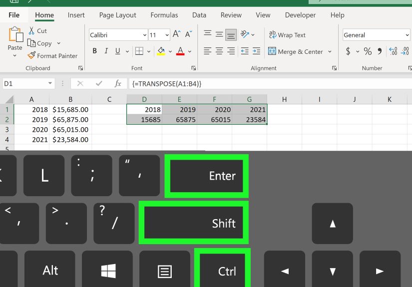
In Microsoft 365 and newer Excel versions with dynamic arrays, the results will “spill” down automatically into a vertical list. In older versions, you typically select the full destination range first (the right height/width), type the formula, then confirm it as an array formula.
Important Notes When Using TRANSPOSE()
- Your output size must match. If your source is 1 row × 6 columns, your result needs 6 rows × 1 column. If you don’t leave enough room, Excel may show a spill/blocked error (newer versions) or simply won’t calculate the way you expect (older versions).
- You can’t edit just one cell in the result. Because it’s produced by a single formula, you usually edit the formula, not individual output cells.
- Want to freeze it as values? Copy the transposed result and Paste Special → Values. That converts the live output into a normal range.
Method 3: Power Query Transpose (Repeatable, Great for Messy Imports)
If you’re transposing a dataset you import regularlylike a weekly CSV export, system report, or vendor filePower Query is your best friend. It lets you build a repeatable set of steps: refresh the data, and the transpose happens again automatically.
Step-by-Step: Transpose with Power Query
- Select your data range and turn it into a table (or use an existing table): Insert → Table
- Go to Data → From Table/Range to open Power Query.
- In Power Query, choose Transform → Transpose.
- If needed, use Transform → Use First Row as Headers to promote the first row into column headers after transposing.
- Click Close & Load to return the transformed data to Excel.
Transpose vs. Unpivot (A Quick Reality Check)
If your goal is “turn columns into rows” for analysis (especially when you have repeated columns like Jan–Dec), you might actually want Unpivot instead of Transpose. Unpivot converts multiple columns into two columns (Attribute and Value), which is often better for PivotTables and charts.
Transpose flips the whole range. Unpivot reshapes the data into a longer, more database-like format. They solve different problemslike a screwdriver vs. a pizza cutter. Both are useful, but one of them is going to make a mess if used incorrectly.
Troubleshooting: Why Your Horizontal-to-Vertical Transpose “Didn’t Work”
- You used Cut instead of Copy: Transpose typically requires copying. If you cut (Ctrl+X), Excel may not allow transpose properly.
- You’re trying to transpose an Excel Table directly: Convert to range first, then transpose.
- Destination area isn’t empty: Excel will overwrite anything in the target range. Pick a blank space.
- The destination area isn’t big enough: A 3×10 range becomes 10×3. Make sure you have room.
- Merged cells block the operation: Unmerge before transposing.
- Formulas behave “differently” after transposing: References may shift because Excel rewrites formulas relative to their new positions. If you want a clean snapshot, paste values while transposing.
Pro Tips for Cleaner Results (and Fewer Spreadsheet Regrets)
Tip 1: Include Labels on Purpose
If your top row contains headers, include them in the copied range so they become row labels after the transpose. If you only copy the data, you may end up with a vertical list that’s missing contextlike a shopping list that just says “12… 47… 3…”
Tip 2: Decide: Do You Need a Snapshot or a Live Link?
- Snapshot (one-time): Paste Special → Transpose
- Live link (updates): =TRANSPOSE(range)
- Repeatable workflow (imports/refresh): Power Query → Transpose
Tip 3: Use a Mini “Method Picker” Cheat Sheet
| Method | Best For | Updates Automatically? | Skill Level |
|---|---|---|---|
| Paste Special → Transpose | Quick flip, small ranges, one-time formatting | No | Beginner |
| TRANSPOSE() formula | Dashboards, templates, “keep it linked” | Yes | Beginner–Intermediate |
| Power Query → Transpose | Recurring imports, bigger transformations, refreshable steps | Yes (on refresh) | Intermediate |
Conclusion
Transposing in Excel is one of those tiny skills that pays rent every month. Whether you need a fast one-time flip (Paste Special), a living, updating mirror of your data (TRANSPOSE), or a repeatable pipeline for messy exports (Power Query), you’ve got a clean way to go from horizontal to vertical without retyping a single cell.
And the next time someone sends you a spreadsheet that’s laid out like a restaurant menu taped sideways to the wall, you can smile confidently… and rotate it like it’s no big deal.
Real-World Transpose Stories (and What They Teach)
Most people don’t learn transposing in a calm, peaceful moment with a fresh cup of coffee and unlimited time. They learn it in the wildusually while muttering, “Why is this laid out like this?” at a spreadsheet that clearly came from a system designed by someone who enjoys chaos.
One common scenario: you download a report where each month is a column across the top, and the template you need to upload into another tool wants months as rows. You try to drag, you try to copy, and suddenly your neatly aligned headings are scattered like confetti. That’s when Paste Special → Transpose feels like magic. The lesson: for a one-time fix, a static transpose is fast and satisfyinglike straightening a crooked picture frame and immediately feeling 12% more organized.
Another scenario shows up in team dashboards. Someone maintains a horizontal “input row” for weekly numbersbecause it’s quick to enter acrossand another sheet needs those same values in a vertical list for charts. People often copy/paste each week (which works until the week they forget, or paste into the wrong place, or paste over the chart labels and wonder why the dashboard looks haunted). That’s when =TRANSPOSE() becomes the hero. The lesson: if you’re repeating a transpose more than once, it’s probably time to use a formula so Excel does the boring part consistently.
Then there’s the “messy import” story: a vendor sends a file every Friday that’s always… almost the same, but not quite. Sometimes there’s an extra blank column. Sometimes the header row shifts. Sometimes you get a surprise “TOTAL” line like a jump scare. Manually transposing each week becomes a ritual of minor suffering. Power Query shines here because you can define steps (clean, transpose, promote headers, load) and then just refresh. The lesson: when the source data is unpredictable or recurring, automation beats heroics.
You’ll also run into the “transpose ate my formulas” moment. Maybe your original horizontal row includes formulas pulling from other cells. After transposing, the formulas might still workbut they might also change their references in ways you didn’t expect, because Excel is trying to be “helpful” about relative references. If your goal is to capture the results, not preserve the logic, paste values while transposing. The lesson: decide whether you’re moving answers or moving math.
Finally, there’s the simple emotional win: the first time you use transpose correctly, you feel like you just learned a secret handshake. It’s not flashy. Nobody throws a parade. But suddenly you can reshape data layouts in secondsand that’s the kind of quiet superpower that makes Excel feel less like a monster and more like a tool.