How to Highlight Alternate Rows in Excel (Every Other Row)

Ever stare at an Excel sheet so long the rows start to blur into a single, judgmental gray rectangle?
Congratsyou’ve discovered why “zebra striping” (highlighting every other row) is one of the simplest, most effective
ways to make data easier to read, audit, and present without accidentally summoning a pivot-table demon.

In this guide, you’ll learn multiple reliable ways to highlight alternate rows in Excelusing built-in Table styles,
Conditional Formatting formulas, and a few pro tweaks for real-world annoyances like headers, blank rows, and filtered lists.
We’ll keep it practical, a little funny, and 100% focused on results.

Why alternate-row shading matters (beyond looking fancy)

• Readability: Your eyes track rows faster when there’s subtle banding.
• Fewer mistakes: It’s harder to copy the wrong row when the visual separation is clear.
• Better presentations: Clean formatting makes reports feel intentional, not “I exported this five minutes ago.”
• Scales with data: With the right method, new rows inherit the pattern automatically.

Method 1 (fastest): Format as a Table with Banded Rows

If your data is a list (columns with headers and rows of records), turning it into an Excel Table is the easiest
way to get alternate row shading that stays consistent as you sort, filter, and add rows.

Step-by-step: Apply banded rows with a Table style

1. Select any cell inside your dataset (or highlight the full range).
2. Go to Home > Format as Table.
3. Pick a style you like and confirm the range.
4. Make sure My table has headers is checked if you have header labels.
5. Click anywhere in the table, then go to Table Design (or Table) and check Banded Rows.

Why Tables are awesome for alternating rows

• Automatic expansion: New rows added at the bottom inherit the shading.
• Filtering-friendly: Table formatting plays nicely with filters and sorting.
• Bonus features: Built-in filter arrows, structured references, and quick totals.

When NOT to use a Table

Tables are perfect for clean lists. But if your sheet is more of a “Franken-grid” (multiple sections, spaced-out blocks,
custom layouts), Conditional Formatting is usually a better fit.

Method 2 (most flexible): Conditional Formatting to shade every other row

Conditional Formatting is the go-to when you want alternate row highlighting on a specific range, custom colors,
or patterns that adapt to changing datawithout converting anything to a Table.

Basic steps: Highlight every other row with a formula

1. Select the range you want to stripe (example: A2:F200).
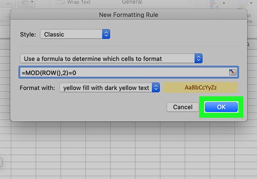
2. Go to Home > Conditional Formatting > New Rule.
3. Choose Use a formula to determine which cells to format.
4. Enter a formula (see options below).
5. Click Format…, choose a Fill color, and click OK.

Formula options (pick your vibe)

Option A: Shade even-numbered rows

Option B: Shade odd-numbered rows

Option C: Same idea, different functions

Example: Start striping after a header row (recommended)

Many sheets have headers in row 1, and the “real” data begins in row 2 (or row 5, or row 37… no judgment).
If you want the first data row to be shaded (or unshaded) consistently, base the pattern on the first row of your selection.

Shade every other row starting from A2 (so A2 is treated as “row 1” of the pattern):

Flip it (shade the alternating rows the other way):

Tip: Replace $A$2 with the top-left cell of your selected data range.
That keeps the pattern anchored even if your range doesn’t start at row 2.

Method 3: Highlight alternate rows but skip blank rows

One common complaint: “Great, now Excel is shading hundreds of empty rows like it’s decorating a runway.”
If your range is larger than your data (common in templates), add a condition that checks whether the row contains data.

Skip blanks by checking a key column

If column A always has something when a row is “real” (like a name, date, ID, etc.), use:

Skip blanks by checking the entire row

If your data might be missing in column A, you can check multiple columns. For example, if your table spans A:F:

This applies shading only when at least one cell in the row contains something.

Method 4: Alternate row shading that behaves with filters (visible rows only)

Here’s the classic “gotcha”: a basic formula like =MOD(ROW(),2)=0 does not “re-count” visible rows
after filtering. So you filter your list… and the striping looks random.

To stripe visible rows only, you can base the pattern on how many visible records appear up to the current row.
One practical approach uses SUBTOTAL to count visible cells in a helper column.

Filtered-friendly formula (example using column A as the “count” column)

Select your data range (example: A2:F200), then use a formula like this:

Notes:

• 3 tells SUBTOTAL to use COUNTA-like behavior (count non-empty visible cells).
• $A$2:$A2 expands as the rule evaluates each row, effectively “counting down the visible list.”
• Choose a column that is reliably filled for each record (IDs are perfect).

If you have blanks in column A, pick a more reliable column (like an ID column) so the visible row count stays accurate.

Method 5: Alternate groups of rows (2-on/2-off, 3-on/3-off, etc.)

Sometimes you don’t want single-row striping. Maybe your data is grouped in pairs or blocks (like two lines per customer,
or a header row + detail row repeating). Conditional Formatting can handle that too.

Shade 2 rows, skip 2 rows (repeat)

Shade 3 rows, skip 1 row (repeat)

The idea: MOD returns the remainder in a repeating cycle. Adjust the cycle length (the divisor) and the threshold
(the “<” number) to create your pattern.

Bonus: Alternate columns instead of rows

If your spreadsheet is more “matrix” than “list,” you might want every other column shaded.

Or anchor the pattern to the first column of your selection:

Troubleshooting: When alternate row highlighting “doesn’t work”

1) Your selection started in the wrong row

If your pattern looks “shifted,” you probably used =MOD(ROW(),2)=0 on a range that starts on an odd/even row
you didn’t intend. Fix it by anchoring to the first row of your selection:

2) Your table style isn’t showing banded rows

In a Table, ensure Banded Rows is turned on under Table Design. Also, if your cells already have fill colors,
they can override the styleclear fills if needed (Home > Fill Color > No Fill).

3) You copied formatting and it “changed”

Conditional Formatting rules are sensitive to relative references. If you copy/paste into a new location,
your anchored cell (like $A$2) may need adjustment. Check:
Home > Conditional Formatting > Manage Rules.

4) You want to override one row’s color

Excel applies Conditional Formatting by rule order. If you need one-off exceptions, create a higher-priority rule
that targets that row (or a condition), then place it above the striping rule. In the rules manager, you can move rules up/down.

Best practices for clean “zebra striping”

• Use subtle fills: Light shading improves readability without fighting your text.
• Pick a reliable anchor cell: Base formulas on the first data row so the pattern stays stable.
• Choose the right method: Tables for structured lists; Conditional Formatting for custom layouts.
• Plan for filters: If filtering is core to your workflow, use a visible-rows approach.

Conclusion

Highlighting every other row in Excel is one of those tiny upgrades that pays rent every day: your data becomes easier to read,
easier to verify, and easier to share without a “Waitwhat row are we on?” group chat.

If you want the simplest “set it and forget it” option, format your range as a Table and use Banded Rows.
If you need precision, patterns, exceptions, or filtered-friendly striping, Conditional Formatting formulas give you full control.
Either way, your spreadsheet will look less like a wall of numbers… and more like you meant to do this on purpose.

Real-World Experiences (and tiny lessons that save big headaches)

In real workplaces, alternate row shading isn’t just “aesthetic.” It’s damage control. People use Excel in the wild for budgets,
inventory logs, attendance sheets, client lists, project trackers, and the legendary “everything file” that somehow becomes a
company’s unofficial database. When those sheets grow past a few dozen rows, the human eye starts doing what it always does:
skipping lines, losing its place, and confidently reading the wrong row with the energy of someone who has never been wrong in their life.

One common scenario: a shared expense tracker. Multiple people add rows over time, and the sheet gets sorted and filtered constantly.
Simple striping (like MOD(ROW(),2)) looks fine… until someone filters the list to “just February” and the shading becomes a patchwork quilt.
That’s when filtered-friendly striping earns its keep. Even if only one person knows how it works, everyone benefits because the sheet stays readable
during the exact moment it matterswhen you’re scanning quickly for the one entry that’s mysteriously double-charged.

Another classic: templates built “for the future,” where the range is pre-formatted down to row 1000. This is well-intentioned and also mildly chaotic.
Without a “skip blanks” condition, your sheet looks like it’s hosting a zebra-themed parade long before the data arrives.
Adding a simple check like $A2<>”” (or COUNTA across the row) keeps the formatting polite. The stripe shows up when the data shows up.
That means less visual noise, fewer confused comments, and fewer coworkers asking if the file is “broken.”

A surprisingly helpful use: review and QA. When someone is auditing a listsay, checking addresses, matching invoice numbers,
or comparing exportsstriped rows make it easier to keep your place while bouncing between columns.
It’s a small ergonomic improvement, like adding labels to your spice jars: not technically required, but you’ll miss it the second it’s gone.

Finally, presentations. When a spreadsheet is going into a meeting (or being screenshared to a dozen tired faces), banded rows quietly signal competence.
It says, “I prepared this,” not “I panicked and exported this from somewhere and hope nobody asks questions.”
And if you’re building recurring reports, a Table style is the low-effort heronew rows inherit formatting automatically, so the report stays consistent
week after week. That consistency reduces mistakes because people know what they’re looking at before they even read the numbers.

The big takeaway from real-world usage: choose the method that matches how the sheet behaves. If it’s a living list that grows, filters, and sorts, Tables shine.
If it’s a custom layout, a dashboard-like range, or something that must follow rules (skip blanks, stripe visible rows, highlight groups), Conditional Formatting is your toolbox.
And if Excel ever makes you feel like you’re overthinking a simple thingdon’t worry. You’re not. You’re just trying to prevent Future You from sending an “Oops” email.